How to use NMA: Introduction with test data

Introduction

This document describes how to use the main functions of NMA to run a single network meta-analysis with survival data.

Example

First load the required packages.

library(NMA)
library(dplyr)
library(purrr)

Settings

Define the BUGS parameters for MCMC. This is not necessary, but recommended, because there are default values for these.

bugs_params <-
  list(
    PROG = "openBugs",  # which version of BUGS to use to run the MCMC
    N.BURNIN = 10,#00,  # number of steps to throw away
    N.SIMS = 150,#0,    # total number of simulations
    N.CHAINS = 2,       # number of chains
    N.THIN = 1,         # thinning rate
    PAUSE = TRUE)

Define the scenario we will use for the analysis.

RANDOM <- FALSE             # is this a random effects model?
REFTX <- "X"                # reference treatment
data_type <- c("hr_data", "surv_bin_data", "med_data") # which type of data to use
label_name <- "label_name"

Read in datasets

The trials data consist of up to 3 separate data frames. A main table, subData, and optional tables for median event time and binary data, survDataMed and survDataBin respectively. Lets read in the each data set separately. In another article we will show how to do this in one function call by including a Reference file in the data folder which contains the meta data of how to read in the study data. If there is no binary or median data used in the NMA then the variables survDataBin and survDataMed are assigned NA.

file_name <- here::here(file.path("inst", "extdata", "survdata_"))

survDataHR <-
  read.csv(paste0(file_name, "hr_test.csv"),
           header = TRUE,
           as.is = TRUE)

survDataBin <-
  tryCatch(
    read.csv(paste0(file_name, "bin_test.csv"),
             header = TRUE,
             as.is = TRUE),
    error = function(e) NA)

survDataMed <-
  tryCatch(
    read.csv(paste0(file_name, "med_test.csv"),
             header = TRUE,
             as.is = TRUE) %>% 
      mutate(medR = floor(medR)),
    error = function(e) NA)

The format of the data should be fairly self-explanatory and looks like the following. For the hazard ratio data

study	base	tx	Lmean	Lse	multi_arm
A	X	Y	-0.5259393	0.1275307	0
B	Y	Z	-0.7133499	0.1437422	0
C	Z	X	-0.3011051	0.1758496	0

For the binary data

study	base	tx	BinR	BinN
A	X	X	34	38
B	X	Y	27	33

and for the median time data

study	base	tx	median	medN	medR
A	X	Y	14.0	45	22
B	Y	Z	18.0	45	22
C	Z	X	15.1	10	5

More information about these data is available in the help documentation which can be accessed with e.g. help(subData).

Build model

The package uses the model in Woods, Hawkins, and Scott (2010) for NMA combining count and hazard ratio statistics in multi-arm trials. For count data, the cumulative count of subjects who have experienced an event in arm \(k\) of study \(s\)

\[ r_{s,k} \sim Bin(F_{s,k}, n_{s,k}) \]

A log cumulative hazard for each trial arm

\[ \ln (H_{s,k}) = \ln ( - \ln (1 - F_{s,k}))) \]

where

\[ \ln (H_{s,k}) = \alpha_s + \beta_k - \beta_b \]

Under an assumption of proportional hazards, the \(\beta_k\) coefficient is equal to the log hazard ratio.

The counts and hazard ratio data can then be used together, placing a normal distribution error on the log HR.

A random effect is included in the model as follows.

\[ \ln (H_{s,k}) = \alpha_s + \beta_k - \beta_b + re_{s,k} - re_{s,b} \]

Now we can create the NMA object to use in the modelling. The workflow is to first create this separately to actually doing the fitting. This then means that we can perform modified fits but we don’t have to redo any of the preparatory work.

nma_model <-
  new_NMA(survDataHR = survDataHR,
          survDataMed = survDataMed,
          survDataBin = survDataBin,
          bugs_params = bugs_params,
          is_random = RANDOM,
          data_type = data_type,
          refTx = REFTX ,
          effectParam = "beta",
          label = "",
          endpoint = "")

nma_model
#> $dat
#> $dat$inits
#> function() {
#>     list(
#>       beta = c(NA, rnorm(nTx - 1, 0, 2)),
#>       sd = 0.1,
#>       alpha = rnorm(nStudies),
#>       d = c(NA, rnorm(nTx - 1, 0, 2)),  ##TODO: can we remove duplication?
#>       mu = rnorm(nStudies),
#>       baseLod = 0) %>% 
#>       .[param_names]  # filter redundant
#>   }
#> <bytecode: 0x0000000016dbfe30>
#> <environment: 0x0000000016db6850>
#> 
#> $dat$survDataHR
#>   study base tx      Lmean       Lse multi_arm Ltx Lbase Lstudy
#> 1     A    X  Y -0.5259393 0.1275307         0   2     1      1
#> 2     B    Y  Z -0.7133499 0.1437422         0   3     2      2
#> 3     C    Z  X -0.3011051 0.1758496         0   1     3      3
#> 
#> $dat$survDataBin
#>   study base tx BinR BinN Btx Bbase Bstudy
#> 1     A    X  X   34   38   1     1      1
#> 2     B    X  Y   27   33   2     1      2
#> 
#> $dat$survDataMed
#>   study base tx median medN medR mediantx medianbase medianstudy
#> 1     A    X  Y   14.0   45   22        2          1           1
#> 2     B    Y  Z   18.0   45   22        3          2           2
#> 3     C    Z  X   15.1   10    5        1          3           3
#> 
#> $dat$bugsData
#> $dat$bugsData$mu_beta
#> [1] 0
#> 
#> $dat$bugsData$prec_beta
#> [1] 1e-06
#> 
#> $dat$bugsData$mu_alpha
#> [1] 0
#> 
#> $dat$bugsData$prec_alpha
#> [1] 1e-06
#> 
#> $dat$bugsData$Lstudy
#> [1] 1 2 3
#> 
#> $dat$bugsData$Ltx
#> [1] 2 3 1
#> 
#> $dat$bugsData$Lbase
#> [1] 1 2 3
#> 
#> $dat$bugsData$Lmean
#> [1] -0.5259393 -0.7133499 -0.3011051
#> 
#> $dat$bugsData$Lse
#> [1] 0.1275307 0.1437422 0.1758496
#> 
#> $dat$bugsData$multi
#> [1] 0 0 0
#> 
#> $dat$bugsData$LnObs
#> [1] 3
#> 
#> $dat$bugsData$nTx
#> [1] 3
#> 
#> $dat$bugsData$nStudies
#> [1] 3
#> 
#> $dat$bugsData$medianStudy
#> [1] 1 2 3
#> 
#> $dat$bugsData$medianTx
#> [1] 2 3 1
#> 
#> $dat$bugsData$medianBase
#> [1] 1 2 3
#> 
#> $dat$bugsData$Bstudy
#> [1] 1 2
#> 
#> $dat$bugsData$Btx
#> [1] 1 2
#> 
#> $dat$bugsData$Bbase
#> [1] 1 1
#> 
#> $dat$bugsData$medianN
#> [1] 45 45 10
#> 
#> $dat$bugsData$medianR
#> [1] 22 22  5
#> 
#> $dat$bugsData$median
#> [1] 14.0 18.0 15.1
#> 
#> $dat$bugsData$medianNObs
#> [1] 3
#> 
#> $dat$bugsData$Bn
#> [1] 38 33
#> 
#> $dat$bugsData$Br
#> [1] 34 27
#> 
#> $dat$bugsData$BnObs
#> [1] 2
#> 
#> 
#> $dat$txList
#> [1] "X" "Y" "Z"
#> 
#> 
#> $data_type
#> [1] "hr_data"       "surv_bin_data" "med_data"     
#> 
#> $bugs_params
#> $bugs_params$PROG
#> [1] "openBugs"
#> 
#> $bugs_params$N.BURNIN
#> [1] 10
#> 
#> $bugs_params$N.SIMS
#> [1] 150
#> 
#> $bugs_params$N.CHAINS
#> [1] 2
#> 
#> $bugs_params$N.THIN
#> [1] 1
#> 
#> $bugs_params$PAUSE
#> [1] TRUE
#> 
#> $bugs_params$run_bugs
#> [1] TRUE
#> 
#> 
#> $bugs_fn
#> function(...)
#>         R2OpenBUGS::bugs(...)
#> <bytecode: 0x0000000016fce310>
#> <environment: 0x0000000016fd2268>
#> 
#> $is_random
#> [1] FALSE
#> 
#> $refTx
#> [1] "X"
#> 
#> $effectParam
#> [1] "beta"
#> 
#> $modelParams
#>        hr_data       med_data                
#>      "totLdev" "totmediandev"    "totresdev" 
#> 
#> $label
#> [1] ""
#> 
#> $endpoint
#> [1] ""
#> 
#> attr(,"class")
#> [1] "nma"
#> attr(,"CALL")
#> attr(,"CALL")$survDataHR
#> survDataHR
#> 
#> attr(,"CALL")$survDataMed
#> survDataMed
#> 
#> attr(,"CALL")$survDataBin
#> survDataBin
#> 
#> attr(,"CALL")$bugs_params
#> bugs_params
#> 
#> attr(,"CALL")$is_random
#> RANDOM
#> 
#> attr(,"CALL")$data_type
#> data_type
#> 
#> attr(,"CALL")$refTx
#> REFTX
#> 
#> attr(,"CALL")$effectParam
#> [1] "beta"
#> 
#> attr(,"CALL")$label
#> [1] ""
#> 
#> attr(,"CALL")$endpoint
#> [1] ""

We can view the network graph.

library(sna)
plotNetwork(nma_model)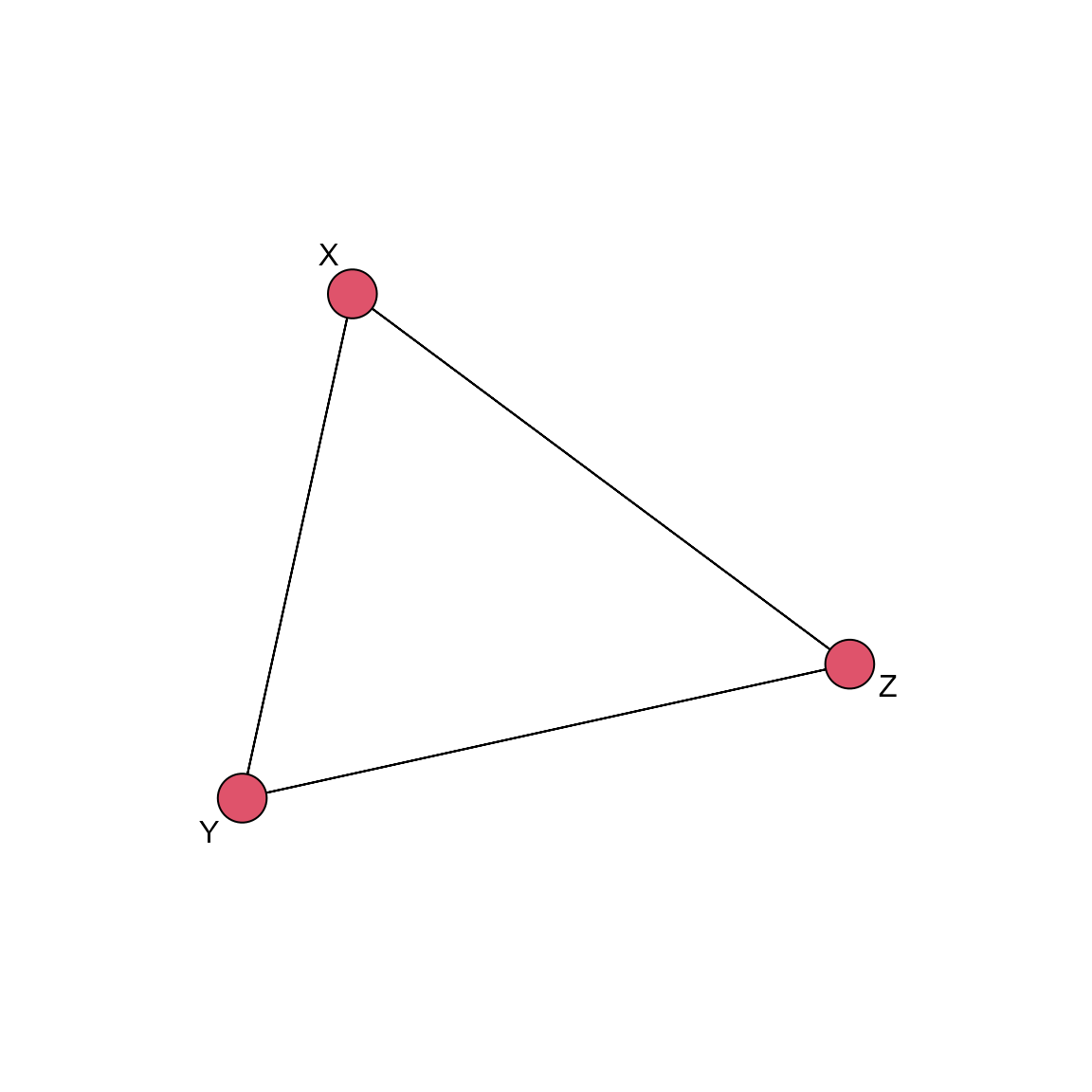

Run MCMC

The NMA MCMC function calls the appropriate BUGS model.

nma_res <- NMA_run(nma_model, save = FALSE)
#> ====== RUNNING BUGS MODEL

nma_res
#> Inference for Bugs model at "C:\Users\n8tha\AppData\Local\Temp\Rtmp4oXQBf/bugs_model.txt", 
#>  2 chains, each with 160 iterations (first 10 discarded)
#>  n.sims = 300 iterations saved
#>               mean    sd  2.5%   25%   50%   75% 97.5% Rhat n.eff
#> beta[2]        0.0   0.9  -1.0  -0.7  -0.4   0.9   1.2  6.4     2
#> beta[3]       -0.7   0.8  -2.2  -1.3  -0.7   0.0   0.6  4.8     2
#> totLdev      132.3  54.9  40.9  87.6 125.8 180.9 249.7  1.0   300
#> totmediandev 226.8 154.8  48.6 123.0 172.8 265.6 558.3  1.1    23
#> totresdev    359.0 198.5  90.5 210.8 310.3 457.3 765.4  1.1    45
#> deviance     500.6 149.6 300.0 390.3 466.9 616.4 799.6  1.1    48
#> 
#> For each parameter, n.eff is a crude measure of effective sample size,
#> and Rhat is the potential scale reduction factor (at convergence, Rhat=1).
#> 
#> DIC info (using the rule, pD = Dbar-Dhat)
#> pD = 143.5 and DIC = 644.1
#> DIC is an estimate of expected predictive error (lower deviance is better).

Reconfigure model

It is simple to modify an existing analysis without repeating the previous steps. For example, we can run the NMA for a random effects rather than a fixed effects model version of the same model.

nma_model2 <-
  NMA_update(nma_model,
             is_random = TRUE)

nma_res2 <- NMA_run(nma_model2, save = FALSE)
#> ====== RUNNING BUGS MODEL

nma_res2
#> Inference for Bugs model at "C:\Users\n8tha\AppData\Local\Temp\Rtmp4oXQBf/bugs_model.txt", 
#>  2 chains, each with 160 iterations (first 10 discarded)
#>  n.sims = 300 iterations saved
#>               mean   sd  2.5%   25%   50%   75% 97.5% Rhat n.eff
#> beta[2]        0.5  0.6  -0.7  -0.1   0.4   1.1   1.6  1.8     5
#> beta[3]       -1.1  0.3  -1.6  -1.4  -1.0  -0.9  -0.6  1.9     4
#> totLdev       28.0 19.8   5.6  14.1  21.5  36.2  76.3  1.3    10
#> totmediandev  52.3 51.1  14.2  27.0  37.1  54.3 200.6  1.3     9
#> totresdev     80.4 62.9  25.9  44.2  60.2  88.1 258.0  1.4     7
#> deviance     145.7 61.0 114.7 118.7 123.8 143.4 355.2  1.0   300
#> 
#> For each parameter, n.eff is a crude measure of effective sample size,
#> and Rhat is the potential scale reduction factor (at convergence, Rhat=1).
#> 
#> DIC info (using the rule, pD = Dbar-Dhat)
#> pD = 27.4 and DIC = 173.2
#> DIC is an estimate of expected predictive error (lower deviance is better).

Plot and tables

BUGS plots are available for diagnosing the performance.

diagnostics(nma_res2, save = TRUE)

Different NMA tables can be created. They can provide a record of the analysis.

write_data_to_file(nma_model)
write_results_table(nma_model, nma_res)

pairwiseTable(nma_model, nma_res)
#>   X                  Y                  Z                 
#> X "1 (1,1)"          "1.47 (0.29,2.72)" "2.11 (0.55,9.12)"
#> Y "0.68 (0.37,3.47)" "1 (1,1)"          "2.29 (1.1,5.08)" 
#> Z "0.47 (0.11,1.82)" "0.44 (0.2,0.91)"  "1 (1,1)"

Currently available NMA plots are a treatment effect forest plot of posterior samples and a rank probability grid.

txEffectPlot(nma_model, nma_res)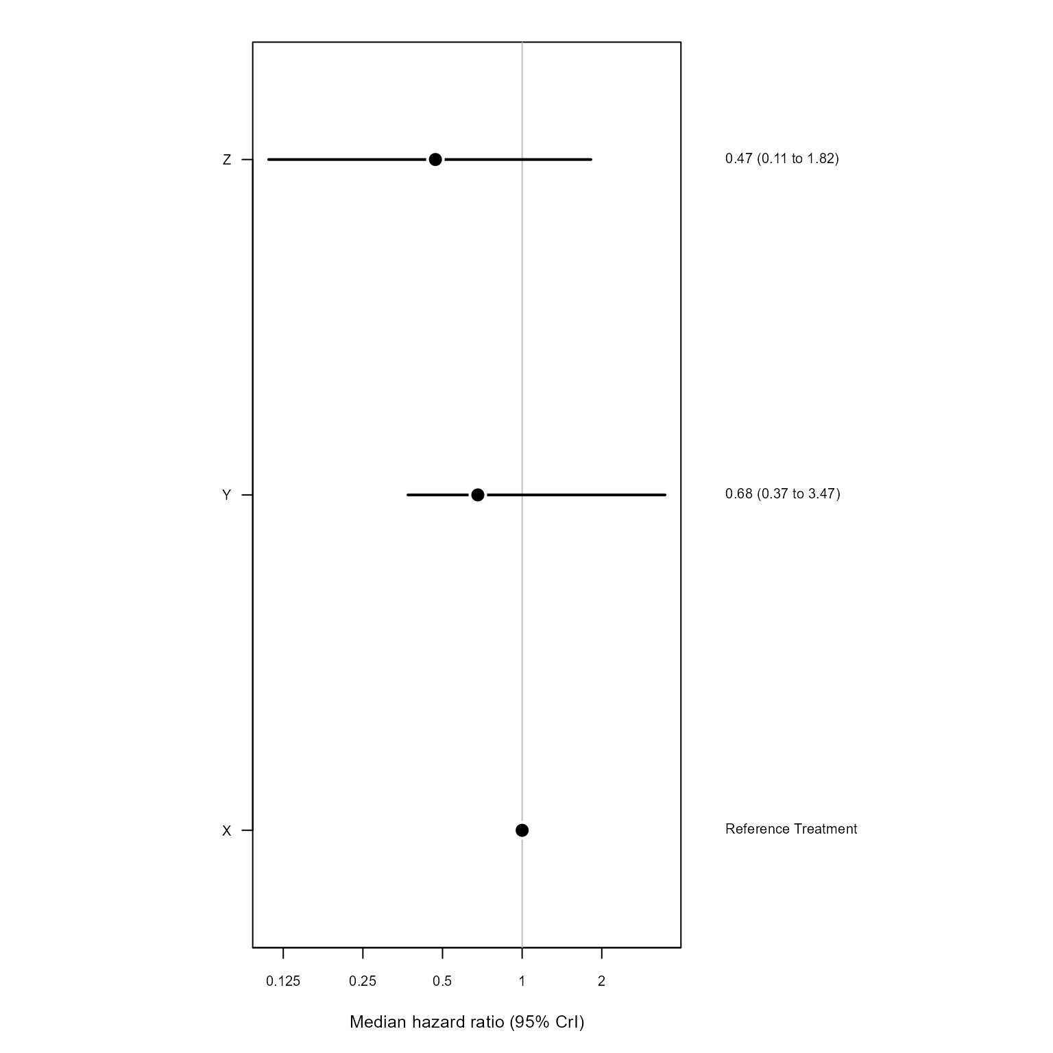

rankProbPlot(nma_model, nma_res)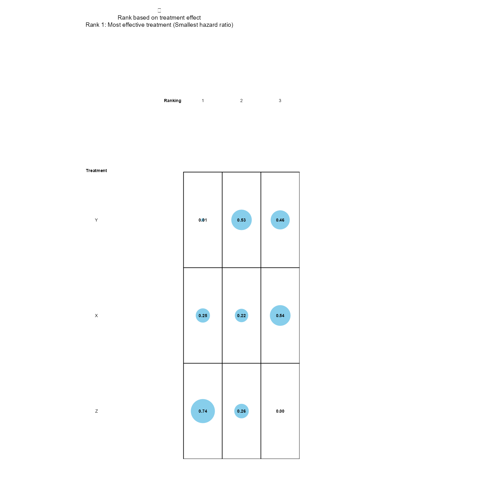

It’s also possible to create all of the BUGS and output plots and table functions together and write to an analysis folder.

nma_outputs(nma_res2, save = TRUE)

References

Woods, Beth S., Neil Hawkins, and David A. Scott. 2010. “Network meta-analysis on the log-hazard scale, combining count and hazard ratio statistics accounting for multi-arm trials: A tutorial.” BMC Medical Research Methodology 10. https://doi.org/10.1186/1471-2288-10-54.