Akaike’s Information Criterion (AIC) and the Bayesian Information Criterion (BIC) provide a useful statistical test of the relative fit of alternative parametric models, and they are usually available as outputs from statistical software. Further details on these are available from (Collett 2013). Measures such as the negative 2 log likelihood are only suitable for comparing nested models, whereby one model is nested within another (for example, one model adds an additional covariate compared to another model). Different parametric models which use different probability distributions cannot be nested within one another. Thus the negative 2 log likelihood test is not suitable for assessing the fit of alternative parametric models. The AIC and BIC allow a comparison of models that do not have to be nested, including a term which penalises the use of unnecessary covariates (these are penalised more highly by the BIC). Generally, it is not necessary to include covariates in survival modelling in the context of an RCT as it would be expected that any important covariates would be balanced through the process of randomisation. However, some parametric models have more parameters than others, and the AIC and BIC take account of these – for example an exponential model only has one parameter and so in comparative terms two parameter models such as the Weibull or Gompertz models are penalised. The AIC and BIC statistics therefore weigh up the improved fit of models with the potentially inefficient use of additional parameters, with the use of additional parameters penalised more highly by the BIC relative to the AIC.
Suppose that we have a statistical model of some data. Let \(k\) be the number of estimated parameters in the model. Let \(\hat{L}\) be the maximized value of the likelihood function for the model. Then the AIC value of the model is the following.
\[
AIC = 2k - 2 \ln({\hat{L}})
\]
Given a set of candidate models for the data, the preferred model is the one with the minimum AIC value.
The BIC is formally defined as
\[
BIC = k \ln(n) - 2 \ln(\widehat{L})
\]
where
\(\hat{L}\) = the maximized value of the likelihood function of the model \(M\), i.e. \(\hat{L} = p(x \mid \widehat{\theta}, M)\), where \(\widehat{\theta}\) are the parameter values that maximize the likelihood function; \(x\) = the observed data; \(n\) = the number of data points in \(x\), the number of observations, or equivalently, the sample size; \(k\) = the number of parameters estimated by the model. For example, in multiple linear regression, the estimated parameters are the intercept, the \(q\) slope parameters, and the constant variance of the errors; thus, \(k = q + 2\).
Relative values
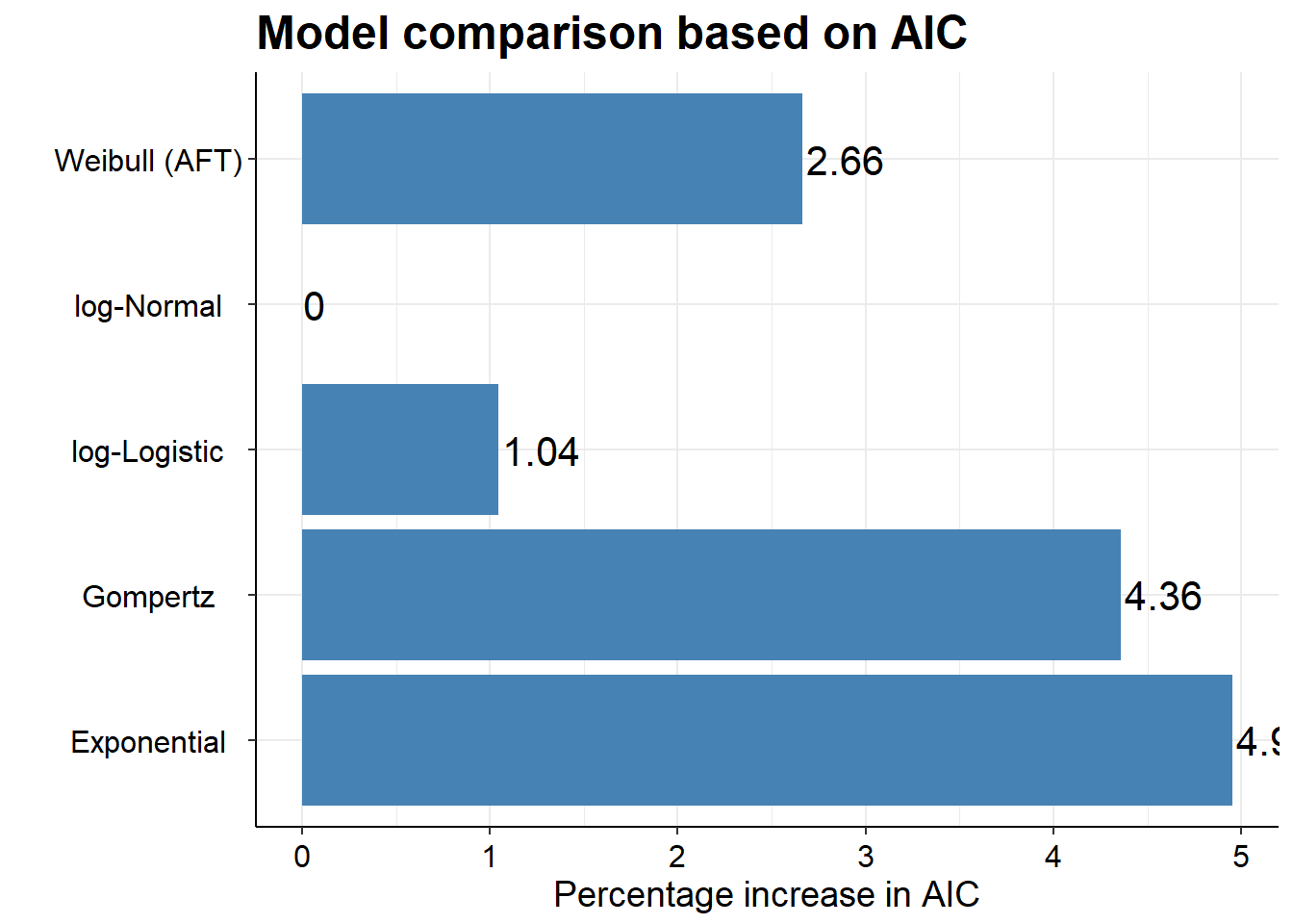
IC values only really make sense when compared between one another i.e relatively. The absolute value is not helpful and depends on the specifics of the model and data.
R example
Cox proportional hazard model
library(survival)test1 <-list(time=c(4,3,1,1,2,2,3), status=c(1,1,1,0,1,1,0), x=c(0,2,1,1,1,0,0), sex=c(0,0,0,0,1,1,1)) # Fit a stratified model fit_ph <-coxph(Surv(time, status) ~ x +strata(sex), test1) AIC(fit_ph)
[1] 8.655313
##TODO: what this difference with AIC()?extractAIC(fit_ph)
[1] 1.000000 8.655313
BIC(fit_ph)
[1] 8.264751
Parametric model with flexsurv
The package flexsurv computes the AIC when it fits a model. This can be accessed by `.\(AIC\) i.e.
library(flexsurv)fitg <-flexsurvreg(formula =Surv(futime, fustat) ~1, data = ovarian, dist ="gengamma")fitg$AIC
[1] 199.8981
For other information criteria statistics it is straightforward to calculate these using the flexsurvreg outpuu. For simplicity we can write a function to do them all at the same time, which we shall call fitstats.flexsurvreg.
Now, the print method for class survHE returns several model fitting summaries.
print(mle)
Model fit for the Exponential model, obtained using Flexsurvreg
(Maximum Likelihood Estimate). Running time: 0.020 seconds
mean se L95% U95%
rate 0.0603838 0.00845542 0.0458911 0.0794534
groupMedium 0.8180219 0.17122084 0.4824352 1.1536086
groupPoor 1.5375232 0.16280169 1.2184378 1.8566087
Model fitting summaries
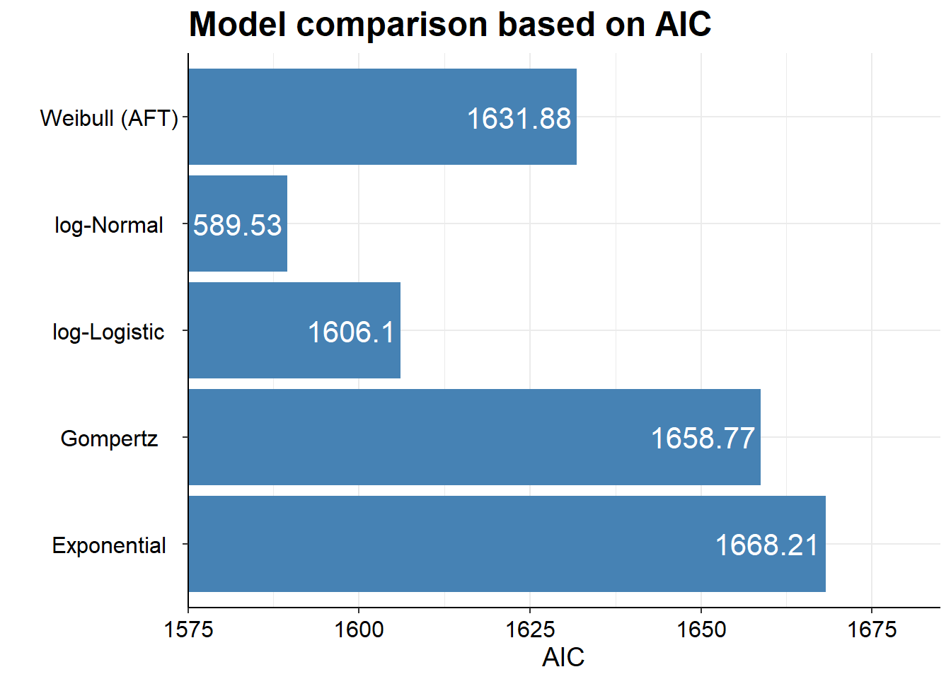
Akaike Information Criterion (AIC)....: 1668.212
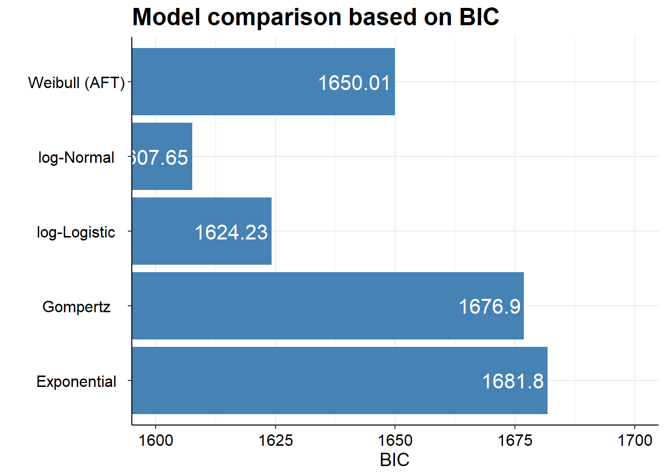
Bayesian Information Criterion (BIC)..: 1681.805
If we wished to access the values directly, perhaps to use in our own code, then we can use
mle$model.fitting
$aic
[1] 1668.212

$bic
[1] 1681.805

$dic
NULL
Further, if we were to fit several different models to compare the IC statistics, which is really the main point of doing it, then survHE also has some nice plotting functions.