devtools::install_github("StatisticsHealthEconomics/blendR")Blended survival curves
Background
We now present a novel approach to alleviate the problem of survival extrapolation with heavily censored data from clinical trials. The main idea is to mix a flexible model (e.g., Cox semiparametric) to fit as well as possible the observed data and a parametric model encoding assumptions on the expected behaviour of underlying long-term survival. The two are ‘’blended’’ into a single survival curve that is identical with the Cox model over the range of observed times and gradually approaching the parametric model over the extrapolation period based on a weight function. The weight function regulates the way two survival curves are blended, determining how the internal and external sources contribute to the estimated survival over time. Further details can be found in (Che, Green, and Baio 2022).
Shiny app
There is an RShiny version of the blendR package for using blended curves interactively in the browser. See here.
R Examples
We need to have the blendR package installed to run this example. This is currently available on GitHub.
In the first example we will use the survHE and INLA packages to fit the external and observed data models, respectively. If the survHE version for doing HMC is missing then install this.
remotes::install_github('giabaio/survHE', ref='hmc')Attach these packages.
We will use the data set available within blendR and so load data in to the current environment.
data("TA174_FCR", package = "blendR")
head(dat_FCR)
# A tibble: 6 × 5
patid treat death death_t death_ty
<int> <int> <int> <dbl> <dbl>
1 1 1 0 32 2.67
2 2 1 0 30.6 2.55
3 3 1 0 28 2.33
4 8 1 0 30 2.5
5 10 1 1 0.458 0.0382
6 11 1 1 1.57 0.131 Fit to the observed data uinsg INLA to obtain the survival object. blendR has a helper function to do this for a piece-wise exponential distribution. The cutpoints argument determines where the points on the survival curve are between which the hazard is constant i.e. an exponential curve.
obs_Surv <- blendR::surv_est_inla(data = dat_FCR,
                                  cutpoints = seq(0, 180, by = 5))
Similarly, we fit the external estimate but first we need to create a synthetic data set consistent with expert judgment. This can be elicited ad-hoc or formally and the process of doing so is a field in itself. Once the values have been elicited then blendR had a function to translate from elicited survival curve constraints to a random sample of survival times. In this case we suppose that we have the information that at time 144 the probability of survival is 0.05.
data_sim <- blendR::ext_surv_sim(t_info = 144,
                                  S_info = 0.05,
                                  T_max = 180)

ext_Surv <- fit.models(formula = Surv(time, event) ~ 1,
                       data = data_sim,
                       distr = "gompertz",
                       method = "hmc",
                       priors = list(gom = list(a_alpha = 0.1,
                                                b_alpha = 0.1)))
SAMPLING FOR MODEL 'Gompertz' NOW (CHAIN 1).
Chain 1:
Chain 1: Gradient evaluation took 0 seconds
Chain 1: 1000 transitions using 10 leapfrog steps per transition would take 0 seconds.
Chain 1: Adjust your expectations accordingly!
Chain 1:
Chain 1:
Chain 1: Iteration:    1 / 2000 [  0%]  (Warmup)
Chain 1: Iteration:  200 / 2000 [ 10%]  (Warmup)
Chain 1: Iteration:  400 / 2000 [ 20%]  (Warmup)
Chain 1: Iteration:  600 / 2000 [ 30%]  (Warmup)
Chain 1: Iteration:  800 / 2000 [ 40%]  (Warmup)
Chain 1: Iteration: 1000 / 2000 [ 50%]  (Warmup)
Chain 1: Iteration: 1001 / 2000 [ 50%]  (Sampling)
Chain 1: Iteration: 1200 / 2000 [ 60%]  (Sampling)
Chain 1: Iteration: 1400 / 2000 [ 70%]  (Sampling)
Chain 1: Iteration: 1600 / 2000 [ 80%]  (Sampling)
Chain 1: Iteration: 1800 / 2000 [ 90%]  (Sampling)
Chain 1: Iteration: 2000 / 2000 [100%]  (Sampling)
Chain 1:
Chain 1:  Elapsed Time: 0.258 seconds (Warm-up)
Chain 1:                0.22 seconds (Sampling)
Chain 1:                0.478 seconds (Total)
Chain 1:

SAMPLING FOR MODEL 'Gompertz' NOW (CHAIN 2).
Chain 2:
Chain 2: Gradient evaluation took 0 seconds
Chain 2: 1000 transitions using 10 leapfrog steps per transition would take 0 seconds.
Chain 2: Adjust your expectations accordingly!
Chain 2:
Chain 2:
Chain 2: Iteration:    1 / 2000 [  0%]  (Warmup)
Chain 2: Iteration:  200 / 2000 [ 10%]  (Warmup)
Chain 2: Iteration:  400 / 2000 [ 20%]  (Warmup)
Chain 2: Iteration:  600 / 2000 [ 30%]  (Warmup)
Chain 2: Iteration:  800 / 2000 [ 40%]  (Warmup)
Chain 2: Iteration: 1000 / 2000 [ 50%]  (Warmup)
Chain 2: Iteration: 1001 / 2000 [ 50%]  (Sampling)
Chain 2: Iteration: 1200 / 2000 [ 60%]  (Sampling)
Chain 2: Iteration: 1400 / 2000 [ 70%]  (Sampling)
Chain 2: Iteration: 1600 / 2000 [ 80%]  (Sampling)
Chain 2: Iteration: 1800 / 2000 [ 90%]  (Sampling)
Chain 2: Iteration: 2000 / 2000 [100%]  (Sampling)
Chain 2:
Chain 2:  Elapsed Time: 0.233 seconds (Warm-up)
Chain 2:                0.212 seconds (Sampling)
Chain 2:                0.445 seconds (Total)
Chain 2:
Now we are nearly ready to fit the blended survival curve. We also need to provide the additional information of how the observed data and external curves are blended together using the beta distribution. That is, we define the blending region min and max and the parameters alpha and beta.
blend_interv <- list(min = 48, max = 150)
beta_params <- list(alpha = 3, beta = 3)
before putting this all together in the blendsurv function.
ble_Surv <- blendR::blendsurv(obs_Surv, ext_Surv, blend_interv, beta_params)A plotting method is available for blendR objects so simply call the following to return the blended survival curve graph.
plot(ble_Surv)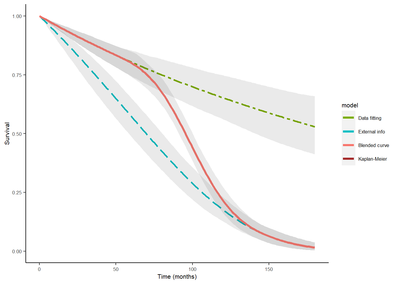
We can alternatively use other survival curves and fitting function for each part of the blended curve. Here we use also fit.model from survHE instead of the INLA fitting function for the observed data model.
obs_Surv2 <- fit.models(formula = Surv(death_t, death) ~ 1,
                        data = dat_FCR,
                        distr = "exponential",
                        method = "hmc")
SAMPLING FOR MODEL 'Exponential' NOW (CHAIN 1).
Chain 1:
Chain 1: Gradient evaluation took 0 seconds
Chain 1: 1000 transitions using 10 leapfrog steps per transition would take 0 seconds.
Chain 1: Adjust your expectations accordingly!
Chain 1:
Chain 1:
Chain 1: Iteration:    1 / 2000 [  0%]  (Warmup)
Chain 1: Iteration:  200 / 2000 [ 10%]  (Warmup)
Chain 1: Iteration:  400 / 2000 [ 20%]  (Warmup)
Chain 1: Iteration:  600 / 2000 [ 30%]  (Warmup)
Chain 1: Iteration:  800 / 2000 [ 40%]  (Warmup)
Chain 1: Iteration: 1000 / 2000 [ 50%]  (Warmup)
Chain 1: Iteration: 1001 / 2000 [ 50%]  (Sampling)
Chain 1: Iteration: 1200 / 2000 [ 60%]  (Sampling)
Chain 1: Iteration: 1400 / 2000 [ 70%]  (Sampling)
Chain 1: Iteration: 1600 / 2000 [ 80%]  (Sampling)
Chain 1: Iteration: 1800 / 2000 [ 90%]  (Sampling)
Chain 1: Iteration: 2000 / 2000 [100%]  (Sampling)
Chain 1:
Chain 1:  Elapsed Time: 0.405 seconds (Warm-up)
Chain 1:                0.278 seconds (Sampling)
Chain 1:                0.683 seconds (Total)
Chain 1:

SAMPLING FOR MODEL 'Exponential' NOW (CHAIN 2).
Chain 2:
Chain 2: Gradient evaluation took 0 seconds
Chain 2: 1000 transitions using 10 leapfrog steps per transition would take 0 seconds.
Chain 2: Adjust your expectations accordingly!
Chain 2:
Chain 2:
Chain 2: Iteration:    1 / 2000 [  0%]  (Warmup)
Chain 2: Iteration:  200 / 2000 [ 10%]  (Warmup)
Chain 2: Iteration:  400 / 2000 [ 20%]  (Warmup)
Chain 2: Iteration:  600 / 2000 [ 30%]  (Warmup)
Chain 2: Iteration:  800 / 2000 [ 40%]  (Warmup)
Chain 2: Iteration: 1000 / 2000 [ 50%]  (Warmup)
Chain 2: Iteration: 1001 / 2000 [ 50%]  (Sampling)
Chain 2: Iteration: 1200 / 2000 [ 60%]  (Sampling)
Chain 2: Iteration: 1400 / 2000 [ 70%]  (Sampling)
Chain 2: Iteration: 1600 / 2000 [ 80%]  (Sampling)
Chain 2: Iteration: 1800 / 2000 [ 90%]  (Sampling)
Chain 2: Iteration: 2000 / 2000 [100%]  (Sampling)
Chain 2:
Chain 2:  Elapsed Time: 0.462 seconds (Warm-up)
Chain 2:                0.26 seconds (Sampling)
Chain 2:                0.722 seconds (Total)
Chain 2:
ext_Surv2 <- fit.models(formula = Surv(time, event) ~ 1,
data = data_sim,
distr = "exponential",
method = "hmc")
SAMPLING FOR MODEL 'Exponential' NOW (CHAIN 1).
Chain 1:
Chain 1: Gradient evaluation took 0 seconds
Chain 1: 1000 transitions using 10 leapfrog steps per transition would take 0 seconds.
Chain 1: Adjust your expectations accordingly!
Chain 1:
Chain 1:
Chain 1: Iteration:    1 / 2000 [  0%]  (Warmup)
Chain 1: Iteration:  200 / 2000 [ 10%]  (Warmup)
Chain 1: Iteration:  400 / 2000 [ 20%]  (Warmup)
Chain 1: Iteration:  600 / 2000 [ 30%]  (Warmup)
Chain 1: Iteration:  800 / 2000 [ 40%]  (Warmup)
Chain 1: Iteration: 1000 / 2000 [ 50%]  (Warmup)
Chain 1: Iteration: 1001 / 2000 [ 50%]  (Sampling)
Chain 1: Iteration: 1200 / 2000 [ 60%]  (Sampling)
Chain 1: Iteration: 1400 / 2000 [ 70%]  (Sampling)
Chain 1: Iteration: 1600 / 2000 [ 80%]  (Sampling)
Chain 1: Iteration: 1800 / 2000 [ 90%]  (Sampling)
Chain 1: Iteration: 2000 / 2000 [100%]  (Sampling)
Chain 1:
Chain 1:  Elapsed Time: 0.183 seconds (Warm-up)
Chain 1:                0.087 seconds (Sampling)
Chain 1:                0.27 seconds (Total)
Chain 1:

SAMPLING FOR MODEL 'Exponential' NOW (CHAIN 2).
Chain 2:
Chain 2: Gradient evaluation took 0 seconds
Chain 2: 1000 transitions using 10 leapfrog steps per transition would take 0 seconds.
Chain 2: Adjust your expectations accordingly!
Chain 2:
Chain 2:
Chain 2: Iteration:    1 / 2000 [  0%]  (Warmup)
Chain 2: Iteration:  200 / 2000 [ 10%]  (Warmup)
Chain 2: Iteration:  400 / 2000 [ 20%]  (Warmup)
Chain 2: Iteration:  600 / 2000 [ 30%]  (Warmup)
Chain 2: Iteration:  800 / 2000 [ 40%]  (Warmup)
Chain 2: Iteration: 1000 / 2000 [ 50%]  (Warmup)
Chain 2: Iteration: 1001 / 2000 [ 50%]  (Sampling)
Chain 2: Iteration: 1200 / 2000 [ 60%]  (Sampling)
Chain 2: Iteration: 1400 / 2000 [ 70%]  (Sampling)
Chain 2: Iteration: 1600 / 2000 [ 80%]  (Sampling)
Chain 2: Iteration: 1800 / 2000 [ 90%]  (Sampling)
Chain 2: Iteration: 2000 / 2000 [100%]  (Sampling)
Chain 2:
Chain 2:  Elapsed Time: 0.163 seconds (Warm-up)
Chain 2:                0.09 seconds (Sampling)
Chain 2:                0.253 seconds (Total)
Chain 2:
ble_Surv2 <- blendR::blendsurv(obs_Surv2, ext_Surv2, blend_interv, beta_params)We can also include the original data Kaplan-Meier in the output plot by simply appending it to the basic plot.
# kaplan-meier
km <- survfit(Surv(death_t, death) ~ 1, data = dat_FCR)

plot(ble_Surv2) +
  geom_line(aes(km$time, km$surv, colour = "Kaplan-Meier"),
            size = 1.25, linetype = "dashed")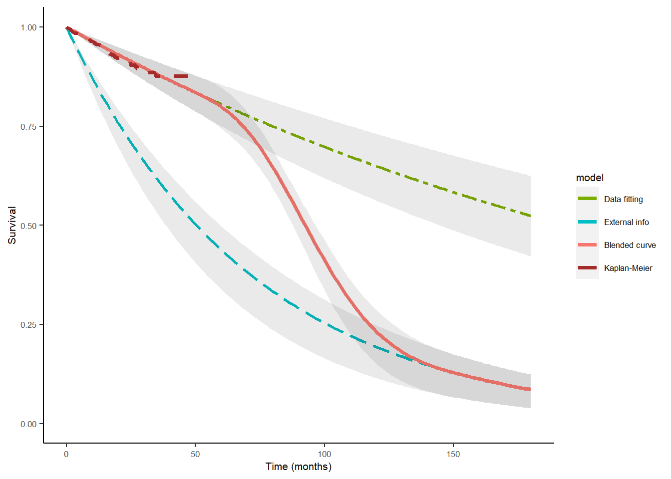
References
Che, Zhaojing, Nathan Green, and Gianluca Baio. 2022. “Blended Survival Curves: A New Approach to Extrapolation for Time-to-Event Outcomes from Clinical Trials in Health Technology Assessment.” Med. Decis. Mak. 25 (1): 0272989X2211345. https://doi.org/10.1177/0272989X221134545.