The median survival time is the length of time from either the date of diagnosis or the start of treatment for a disease, such as cancer, that half of the patients in a group of patients diagnosed with the disease are still alive. In a clinical trial, measuring the median overall survival is one way to see how well a new treatment works. Also called median survival.
Tip
The median is useful but it is the expected or mean survival time that is of particular interest for HTA.
R Examples
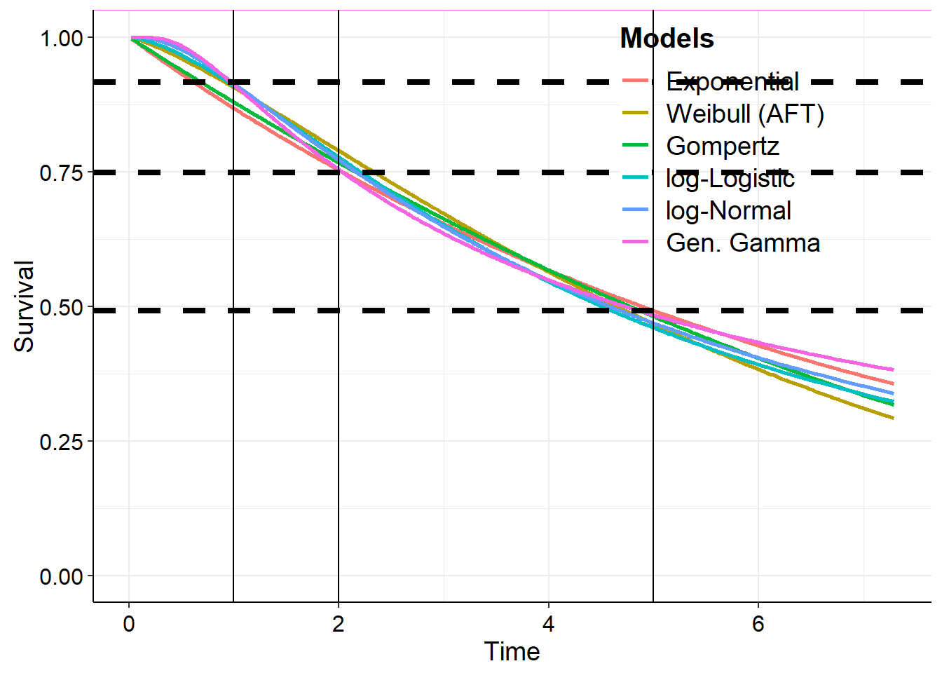
In this example we will see a comparison of survival probabilities at given landmark times as well as the comparison of observed (i.e. based on Kaplan-Meier) and predicted medians (using the respective formula to calculate the median for each distribution) based on fitted models for each of the 6 main distributions we consider.
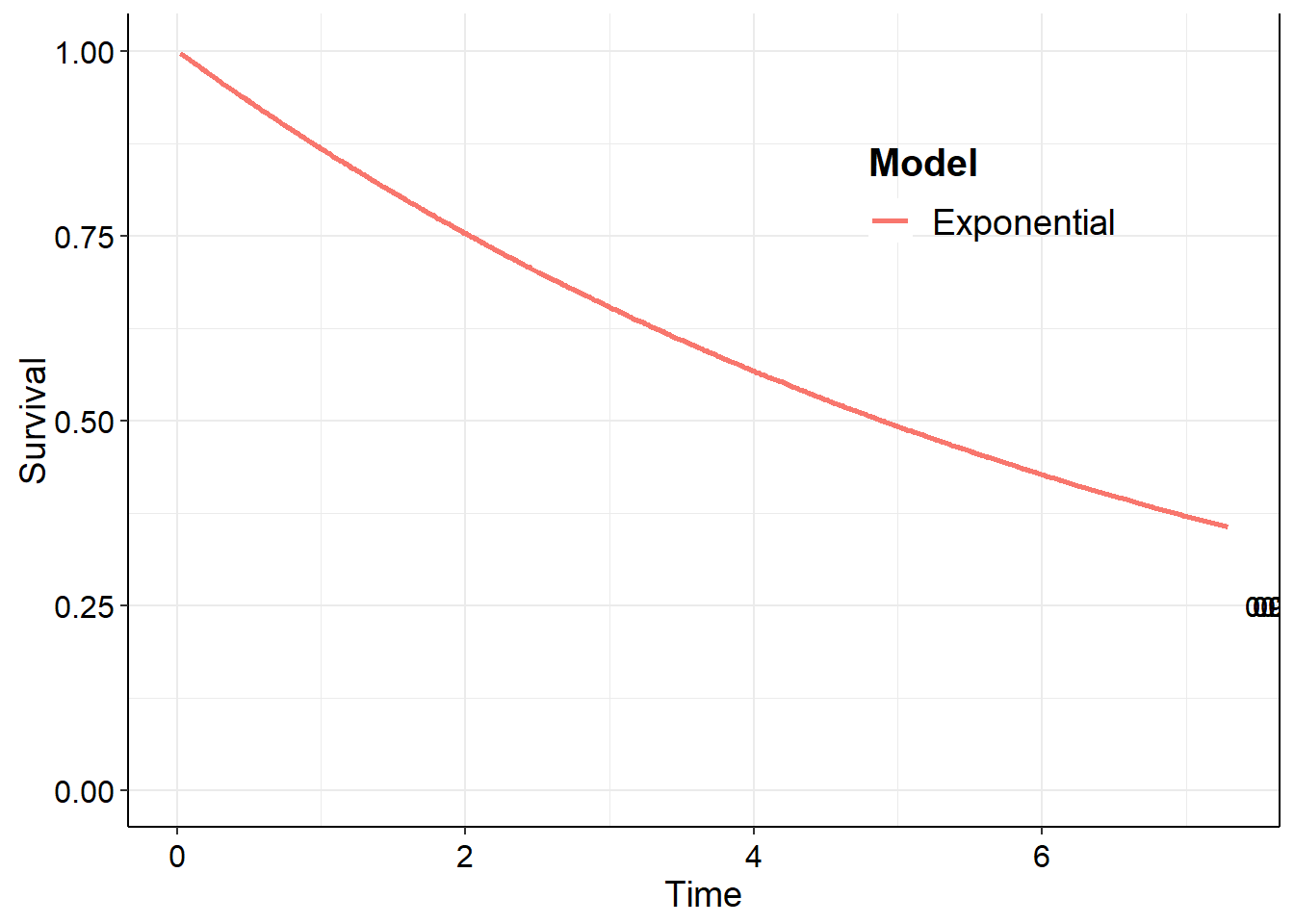
The summary method for a survHE object from the survHE package returns mean survival times, including the median mean survival time (not be be confused with the mean median survival time!). For an exponential model fit with no covariates,
Estimated average survival time distribution*
 mean sd 2.5% median 97.5%
    0  0    0      0     0

*Computed over the range: [0.02192-7.28493] using 1000 simulations.
NB: Check that the survival curves tend to 0 over this range!
Note that this is calculated over a closed range and not the entire time line.
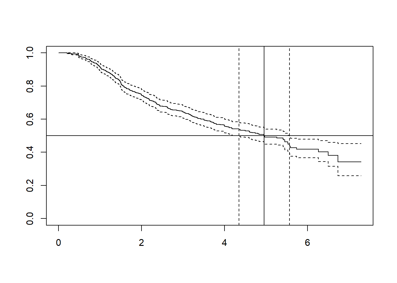
We can compare these parametric estimate with the median survival time from the Kaplan-Meier. This is available from the survHE output in misc$km and the equation
If we denote the median with \(t_{50}\) then to calculate the medians ourselves we can take the fitted coefficient value from the fit.model output and use an inverese of the survival function. In the case of the exponential distribution this is
Which leads to the median \(t_{50} = \alpha\), i.e. simply the shape parameter.
Similarly, the Gompertz distribution median is
\[
(1/b) \log[(-1/\eta) \log(0.5) + 1]
\]
The Weibull distribution median is
\[
\lambda [- \log(0.5)]^{1/k}
\]
The log-normal distribution median is
\[
\exp(\mu)
\]
The gamma distribution has no simple closed form formula for the median.
Simulation-based estimates
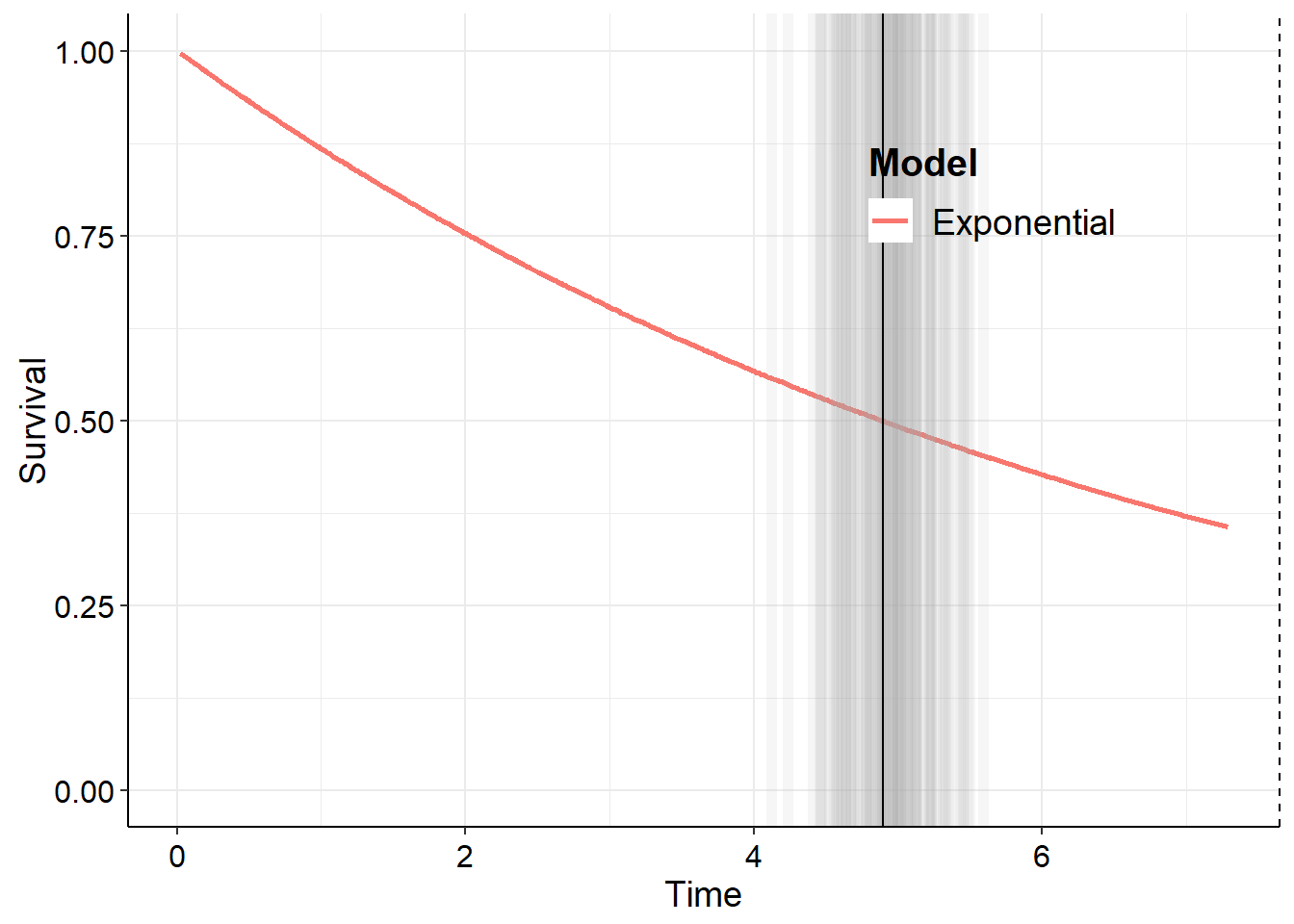
Note that the parameter returned from fit.model is the log of the rate. More generally, we can simulate (multiple) survival curves from the coefficient posterior and estimate the median for each of these. So, sample from the posterior using make.surv() from the survHE package to obtain output for the single curve case as follows.
surv_exp <-make.surv(mle)
The sampled survival curves from make.surv() have slightly different names so let us redefine the median function and then extract the median times.
Warning: Using `size` aesthetic for lines was deprecated in ggplot2 3.4.0.
ℹ Please use `linewidth` instead.
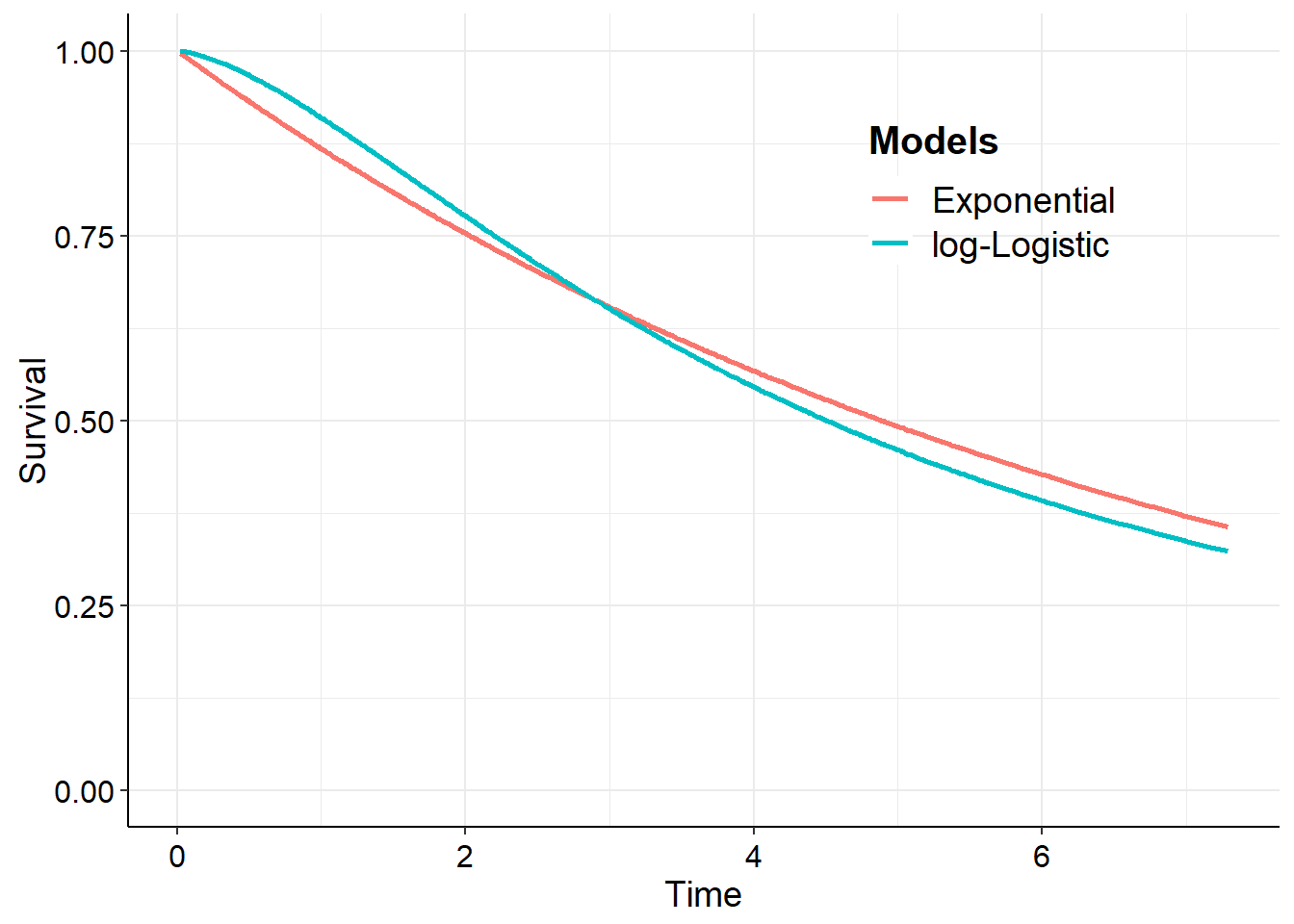
Multiple distributions
In the same way as for a single distribution, we can extend the analysis for multiple distributions at the same time. We show this for exponential and log-logistic distributions. First, fit the models and show the survival curves.
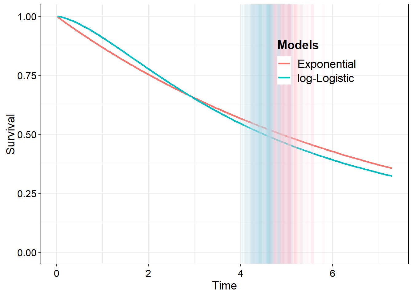
Now we can automatically create functions for all the percentiles of interest by mapping over the vector of probabilities, which returns a list of functions.
Comparing between all distribution fits and Kaplan-Meier
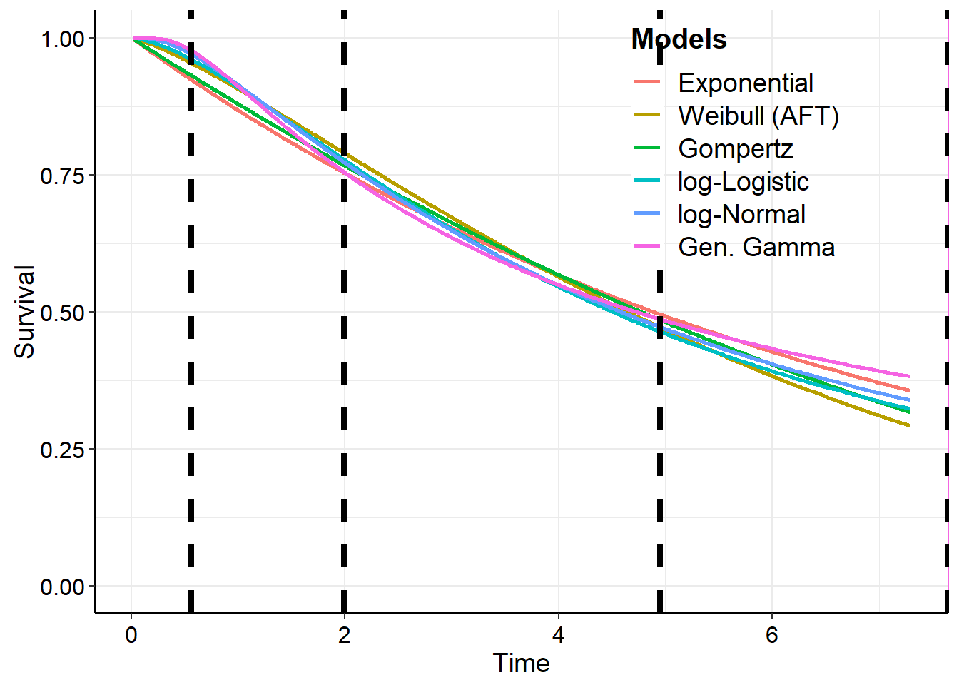
In this section we bring together various things from previous sections. We will do an analysis for all 6 main distributions at the same time and for several percentiles.
First, we fit all of the models and then generate the sample of survival curves.
Warning in min(S[["t"]][S[[sname]] < 0.5]): no non-missing arguments to min;
returning Inf
Warning in min(S[["t"]][S[[sname]] < 0.5]): no non-missing arguments to min;
returning Inf
Warning in min(S[["t"]][S[[sname]] < 0.5]): no non-missing arguments to min;
returning Inf
Warning in min(S[["t"]][S[[sname]] < 0.5]): no non-missing arguments to min;
returning Inf
Warning in min(S[["t"]][S[[sname]] < 0.5]): no non-missing arguments to min;
returning Inf
Warning in min(S[["t"]][S[[sname]] < 0.5]): no non-missing arguments to min;
returning Inf
Warning in min(S[["t"]][S[[sname]] < 0.5]): no non-missing arguments to min;
returning Inf
Warning in min(S[["t"]][S[[sname]] < 0.5]): no non-missing arguments to min;
returning Inf
Warning in min(S[["t"]][S[[sname]] < 0.5]): no non-missing arguments to min;
returning Inf
Warning in min(S[["t"]][S[[sname]] < 0.5]): no non-missing arguments to min;
returning Inf
Warning in min(S[["t"]][S[[sname]] < 0.5]): no non-missing arguments to min;
returning Inf
Warning in min(S[["t"]][S[[sname]] < 0.5]): no non-missing arguments to min;
returning Inf
Warning in min(S[["t"]][S[[sname]] < 0.5]): no non-missing arguments to min;
returning Inf
Warning in min(S[["t"]][S[[sname]] < 0.5]): no non-missing arguments to min;
returning Inf
Warning in min(S[["t"]][S[[sname]] < 0.5]): no non-missing arguments to min;
returning Inf
Warning in min(S[["t"]][S[[sname]] < 0.5]): no non-missing arguments to min;
returning Inf
Warning in min(S[["t"]][S[[sname]] < 0.5]): no non-missing arguments to min;
returning Inf
Warning in min(S[["t"]][S[[sname]] < 0.5]): no non-missing arguments to min;
returning Inf
[[1]]
[[1]]$Exponential
 [1] 4.966553 4.827020 4.883045 5.628640 5.035439 5.292257 5.089955 4.804941
 [9] 4.982657 4.810618

[[1]]$`Weibull (AFT)`
 [1] 4.743420 4.493634 4.745278 4.337766 4.626728 4.657598 4.464190 4.717536
 [9] 4.582725 4.676070

[[1]]$Gompertz
 [1] 4.046255 4.358841 4.227582 4.307995 4.373330 3.678017 3.759001 4.338441
 [9] 3.509706 3.523070

[[1]]$`log-Logistic`
 [1] 5.013626 4.066543 4.580682 4.959065 4.212073 4.036718 4.555648 4.273214
 [9] 4.446469 4.491434

[[1]]$`log-Normal`
 [1] 4.657814 4.132980 4.784933 5.107095 4.871923 4.441884 4.251263 4.747124
 [9] 4.518871 4.463943

[[1]]$`Gen. Gamma`
 [1] NA NA NA NA NA NA NA NA NA NA


[[2]]
[[2]]$Exponential
median    upp    low
   Inf    Inf    Inf

[[2]]$`Weibull (AFT)`
median    upp    low
   Inf    Inf    Inf

[[2]]$Gompertz
median    upp    low
   Inf    Inf    Inf

[[2]]$`log-Logistic`
median    upp    low
   Inf    Inf    Inf

[[2]]$`log-Normal`
median    upp    low
   Inf    Inf    Inf

[[2]]$`Gen. Gamma`
median    upp    low
   Inf    Inf    Inf