Proportional Hazard Modelling

Introduction

The purpose of the CPH model is to evaluate simultaneously the effect of several factors on survival. It allows us to examine how specified factors influence the rate of a particular event happening at a particular point in time. This rate is commonly referred as the hazard rate.

The Cox model is expressed by the hazard function denoted by \(h(t)\). The hazard function can be interpreted as the risk of dying at time \(t\).

It can be estimated as follow:

\[ h(t) = h_0(t) \times \exp (\beta_1 x_1 + \beta_2 x_2 + \cdots + \beta_p x_p) \]

where

\(h_0\) is the baseline hazard corresponding to the value of the hazard if all of the \(x_i\) are equal to zero.
Each \(\exp(\beta_i)\) are the hazard ratios. Id HR < 1the there is a reduction in the hazard and if HR > 1 then there is an increase in the hazard.

Example in R

We will use the standard package survival for this and the package survminer which has some nice plotting functions.

library("survival")
library("survminer")

Load the data

data("lung")

Warning in data("lung"): data set 'lung' not found

head(lung)

  inst time status age sex ph.ecog ph.karno pat.karno meal.cal wt.loss
1    3  306      2  74   1       1       90       100     1175      NA
2    3  455      2  68   1       0       90        90     1225      15
3    3 1010      1  56   1       0       90        90       NA      15
4    5  210      2  57   1       1       90        60     1150      11
5    1  883      2  60   1       0      100        90       NA       0
6   12 1022      1  74   1       1       50        80      513       0

and compute a univariate Cox model

res.cox <- coxph(Surv(time, status) ~ sex, data = lung)
summary(res.cox)

Call:
coxph(formula = Surv(time, status) ~ sex, data = lung)

  n= 228, number of events= 165 

       coef exp(coef) se(coef)      z Pr(>|z|)   
sex -0.5310    0.5880   0.1672 -3.176  0.00149 **
---
Signif. codes:  0 '***' 0.001 '**' 0.01 '*' 0.05 '.' 0.1 ' ' 1

    exp(coef) exp(-coef) lower .95 upper .95
sex     0.588      1.701    0.4237     0.816

Concordance= 0.579  (se = 0.021 )
Likelihood ratio test= 10.63  on 1 df,   p=0.001
Wald test            = 10.09  on 1 df,   p=0.001
Score (logrank) test = 10.33  on 1 df,   p=0.001

For a multivariate Cox model it is a simple extension

res.cox <- coxph(Surv(time, status) ~ age + sex + ph.ecog, data =  lung)
summary(res.cox)

Call:
coxph(formula = Surv(time, status) ~ age + sex + ph.ecog, data = lung)

  n= 227, number of events= 164 
   (1 observation deleted due to missingness)

             coef exp(coef)  se(coef)      z Pr(>|z|)    
age      0.011067  1.011128  0.009267  1.194 0.232416    
sex     -0.552612  0.575445  0.167739 -3.294 0.000986 ***
ph.ecog  0.463728  1.589991  0.113577  4.083 4.45e-05 ***
---
Signif. codes:  0 '***' 0.001 '**' 0.01 '*' 0.05 '.' 0.1 ' ' 1

        exp(coef) exp(-coef) lower .95 upper .95
age        1.0111     0.9890    0.9929    1.0297
sex        0.5754     1.7378    0.4142    0.7994
ph.ecog    1.5900     0.6289    1.2727    1.9864

Concordance= 0.637  (se = 0.025 )
Likelihood ratio test= 30.5  on 3 df,   p=1e-06
Wald test            = 29.93  on 3 df,   p=1e-06
Score (logrank) test = 30.5  on 3 df,   p=1e-06

We can visualise the output as follows.

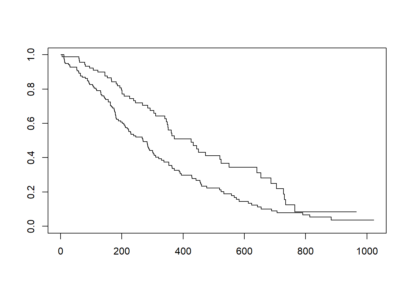
fit <- survfit(Surv(time, status) ~ sex, data = lung)

# base R
plot(fit)

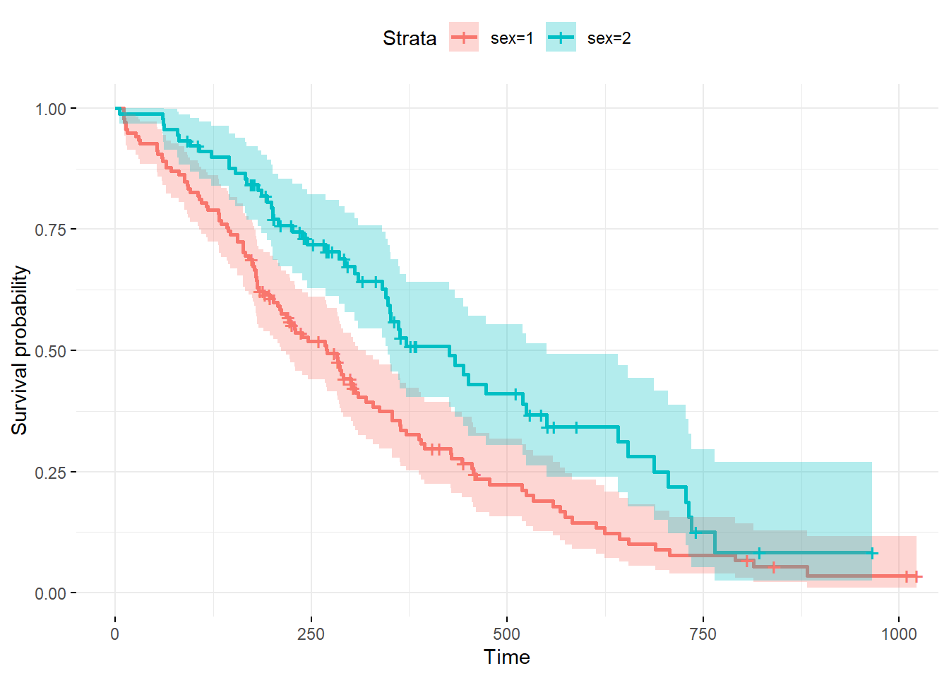
# ggplot2
ggsurvplot(fit, conf.int = TRUE,
           ggtheme = theme_minimal(), data = lung)